3.1 矩阵
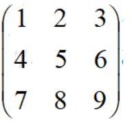
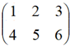
矩阵一般有M行N列,比如:

表示3行3列的矩阵
表示2行3列的矩阵
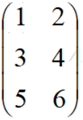
表示3行2列的矩阵
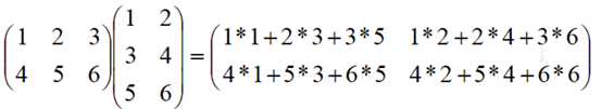
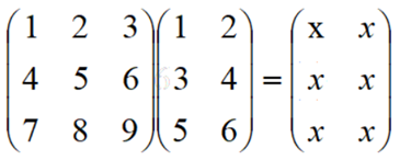
如果两个矩阵的连接,有个规定:第1个矩阵的列数必须和第二个矩阵的行数是一样的
2行3列 * 3行2列 = 2行2列
3行3列 * 3行2列 = 3行2列
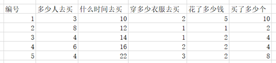
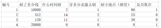
一行称为一个样本(sample),一列称为一个特征(feature)
根据不同的样本建立表格(采样)
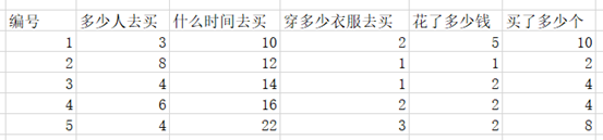
建立式子:
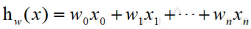
所以上面的式子可以理解为1个1行N列的矩阵,乘以一个N行1列的矩阵
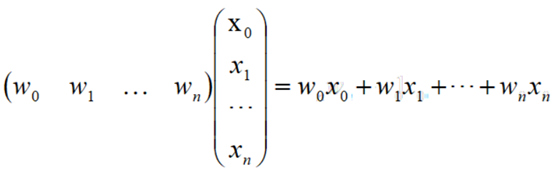
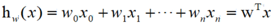
最终的式子描述为
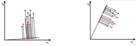
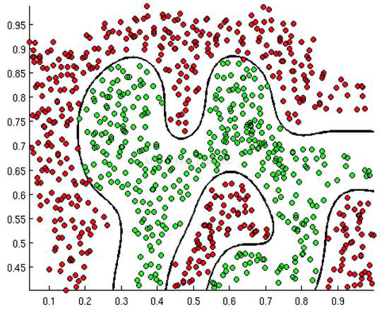
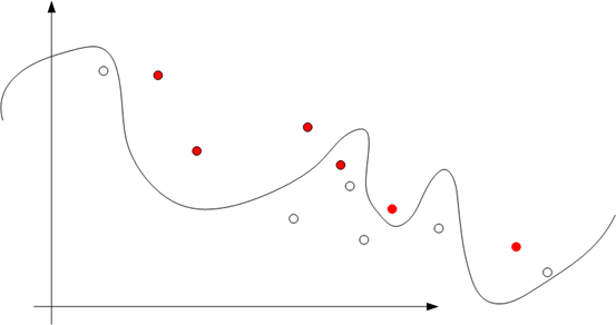
3.2 降维
3 分类清晰
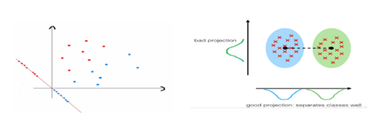
所以,降维的方向很重

这里是把3维降到2维
3.3 导入数据
首先需要安装python做数据分析的包numpy、pandas、matplotlib
pip install numpy
pip install pandas
pip install matplotlib

pip install numpy -i http://pypi.douban.com/simple --trusted-host pypi.douban.com
pip install pandas -i http://pypi.douban.com/simple --trusted-host pypi.douban.com
pip install matplotlib -i http://pypi.douban.com/simple --trusted-host pypi.douban.com
导入对应的库
# 导入python中需要的包
import numpy as np # 数学运算库
import pandas as pd # 数据分析库
import matplotlib.pyplot as plt # 绘图库
需要简单运行一下,确保能够正常导入这几个库
# 读入数据 data = pd.read_csv('creditcard.csv')
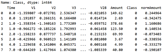
# 显示前8行数据 print(data.head(8))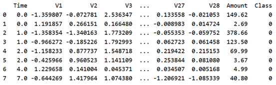
Class表示分类的类别。0表示正常交易,1表示出现欺诈行为
3.4 类别的数据统计
统计一下Amount中有多少0,多少个1
plt.rcParams['font.sans-serif'] = ['SimHei']
# 统计Class特征为0和为1的样本分别有多少个
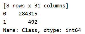
count_classes = pd.value_counts(data['Class'])
print(count_classes)
# 0 284315
# 1 492
# 绘制图形分析数据
count_classes.plot(kind='bar') # 绘制柱状图
plt.title('信用卡欺诈统计数据') # 图的标题
plt.xlabel('分类') # x轴的标签
plt.ylabel('数量') # y轴的标签
#plt.show()
plt.savefig('img/1.png')

3.5 数据标准化、归一化
高斯分布、正态分布
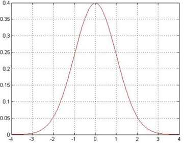
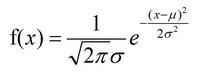
其中 u 是均值,σ是标准差
当 u=0,σ=1,则为标准正态分布
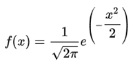
标准正态分布,称为(0, 1)的正态分布,平均值为0,方差是1
数据处理后的目标就是服从标准的正态分布
pip install scikit-learn -i http://pypi.douban.com/simple --trusted-host pypi.douban.com# 导入标准正态分布的表
from sklearn.preprocessing import StandardScaler
# reshape 重新调整数据的行和列数 将数据转换为矩阵
# 参数1 转换后的矩阵有多少行 -1表示不看重行数 行数=总数/列数
# 参数2 转换后的矩阵有多少列 -1表示不看重列数 列数=总数/行数
reshape = data['Amount'].values.reshape(-1, 1)
# 把数据按标准正态分布的方式转换为均值为0 方差为1 的数据
data['normAmount'] = StandardScaler().fit_transform(reshape)
# drop()删除数据
# 参数1 要删除的特征列
# 参数2 axis指定是删除行还是删除列 0代表行 1代表列
data = data.drop(['Time', 'Amount'], axis=1)
print(data.head(8))
运行程序,现在Amount特征就被删除了,添加了normAmount特征
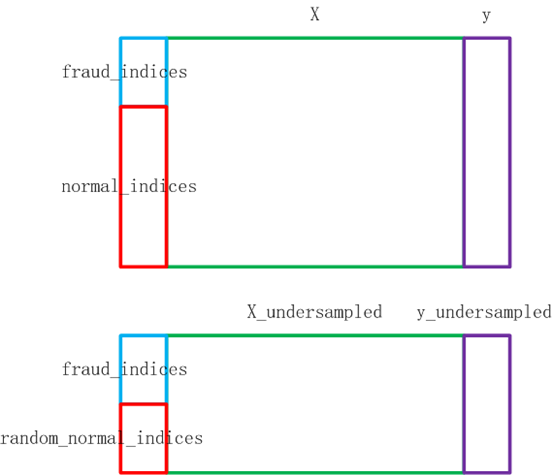
3.6 OverSampled 和 UnderSampled
UnderSampled:欠采样
1 把0的数据量减少为1的数据量,从多的数据量中筛选一部分数据。UnderSampled
2 把1的数据量增加到0的数据量,从小的数据量中生成数据。OverSampled
首先进行UnderSampled
# X拿到非Class的特征数据
X = data.loc[:, data.columns != 'Class']
# y拿到Class的特征数据
y = data.loc[:, data.columns == 'Class']

# 计算少数类别的样本有多少个
number_records_fraud = len(data[data.Class == 1])
# 求出少数类别样本对应的索引值
fraud_indices = np.array(data[data.Class == 1].index)
#print(fraud_indices)
# 求出多数类别样本对应的索引值
normal_indices = np.array(data[data.Class == 0].index)
#print(normal_indices)
# 从多数类别的样本索引normal_indices中随机筛选fraud_indices个
# choice(a, size=None, replace=True, p=None)
# 参数1 a 样本集
# 参数2 size 选择多少个
# 参数3 replace 是否替换原来的数据
random_normal_indices = np.random.choice(normal_indices, number_records_fraud, replace=False)
#print(len(random_normal_indices)) # 492
# 把random_normal_indices和fraud_indices混合起来作为后面的undersampled的学习样本
# concatenate(arrays, axis=None, out=None)
# 参数1 元组 要整合的所有的数据
# 参数2 axis 整合的方向 0代表行的整合 492行+492行=984行
under_sample_indices = np.concatenate((random_normal_indices, fraud_indices), axis=0)
#print(len(under_sample_indices)) # 984

# iloc根据索引得到数据
under_sample_data = data.iloc[under_sample_indices, :]
#print(len(under_sample_data)) # 984

# 得到X_undersampled和y_undersampled
# X_undersampled从undersampled数据中拿到非Class特征
X_undersampled = under_sample_data.iloc[:, data.columns != 'Class']
# y_undersampled从undersampled数据中拿到Class特征
y_undersampled = under_sample_data.iloc[:, data.columns == 'Class']
#print(y_undersampled)
# 汇总
print('undersampled中所有样本的个数:', len(under_sample_data)) # 984
print('undersampled中正常样本的个数:', len(random_normal_indices)) # 492
print('undersampled正常样本占的比例:', len(random_normal_indices)/len(under_sample_data)) # 0.5
print('undersampled中欺诈样本的个数:', len(fraud_indices)) # 492
print('undersampled欺诈样本占的比例:', len(fraud_indices)/len(under_sample_data))#0.5
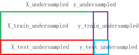
3.7 UnderSampled样本划分训练集、验证集、测试集
通过训练集训练出模型,使用验证集检验模型。交替训练集和验证集,得出比较靠谱的模型
接下来需要对UnderSampled的数据进行划分,划分成训练集+验证集+测试集
from sklearn.model_selection import train_test_split
# 划分训练集+验证集+测试集
# 参数1 所要划分的样本的特征集
# 参数2 所要划分的样本的结果集
# 参数3 test_size 测试集占所有样本的比例
# 参数4 random_state 划分的结果是否随机
# 0 每次划分的结果都不同
# 1 每次划分的结果都相同
# 返回值1 特征的训练集+验证集
# 返回值2 特征的测试集
# 返回值3 结果的训练集+验证集
# 返回值4 结果的测试集
X_train_undersampled, X_test_undersampled, y_train_undersampled, y_test_undersampled = \
train_test_split(X_undersampled, y_undersampled, test_size=0.3, random_state=0)
print('对undersampled数据进行划分,训练集+验证集数据长度是:', len(y_train_undersampled)) # 688
print('对undersampled数据进行划分,测试集数据长度是:', len(y_test_undersampled)) # 296
print('总共的数据量是:', len(y_train_undersampled) + len(y_test_undersampled)) # 984
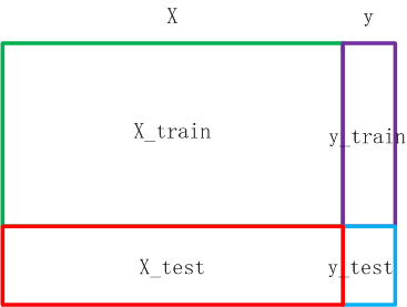
X_train, X_test, y_train, y_test = \
train_test_split(X, y, test_size=0.3, random_state=0)
print('对原始数据进行划分,训练集+验证集数据长度是:', len(y_train)) # 199364
print('对原始数据进行划分,测试集数据长度是:', len(y_test)) # 85443
print('总共的数据量是:', len(y_train) + len(y_test)) # 284807
3.8 训练的目的是什么

如果可以计算出w权重值,当下一个样本来到的时候,就可以进行分类
这个是二分类的基本思路(逻辑回归)
当前案例中,要提高准确率是非常简单的,只要把所有的样本都划分为正常交易记录即可
总共有284807个样本,其中284315个正常样本,492个欺诈样本
如果把所有样本都划分为正常样本,则准确率为 284315 / 284807 = 99.8%
思路:划分正确的样本占总的正确样本的比例

水平轴表示预测值。1表示预测为欺诈行为,0表示预测为正常行为
垂直轴表示原本值。1表示原本为欺诈行为,0表示原本为正常行为
Positive预测为欺诈行为(正类1),Negative预测为正常行为(负类0)
TP:True Positive。预测正确True,预测为欺诈行为Positive。原本是欺诈行为。右下角象限
FP:False Positive。预测错误False,预测为欺诈行为Positive。原本是正常行为。右上角象限
TN:True Negative。预测正确True,预测为正常行为Negative,原本是正常行为。左上角象限
FN:False Negative。预测错误False,预测为正常行为Negative。原本为欺诈行为。左下角象限
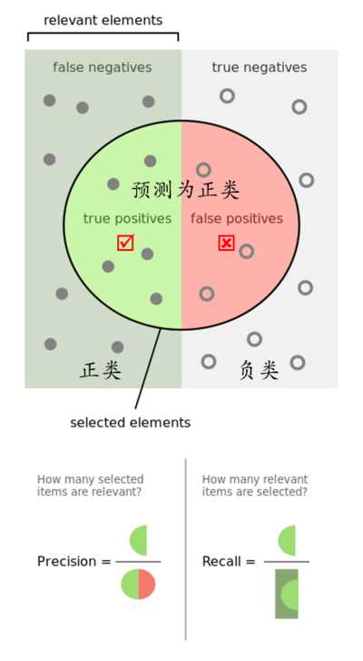
Recall召回率:TP / (TP + FN) = 右下 / (右下 + 左下)
Precision精确率:TP / (TP + FP) = 右下 / (右下 + 右上)
Accuracy准确率:(TP + TN) / (TP + TN + FP + FN) = (右下 + 左上) / (右下 + 右上 + 左下 + 左上)
明天有可能下雨,你要不要带伞?
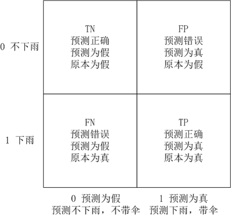
召回率 = TP / (TP + FN) = 右下 / (右下 + 左下) = 下雨了,带伞没?
精确率 = TP / (TP + FP) = 右下 / (右下 + 右上) = 带伞了,下雨没?
明天可能是女朋友生日,要不要送礼?
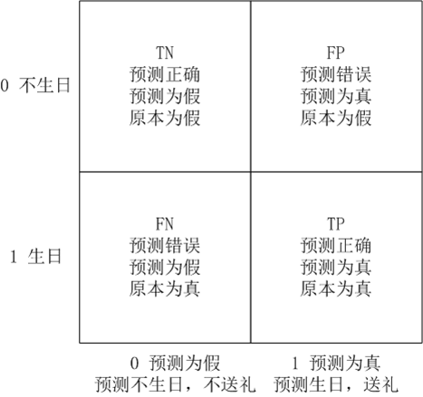
召回率 = TP / (TP + FN) = 右下 / (右下 + 左下) = 生日了,送礼没?
精确率 = TP / (TP + FP) = 右下 / (右下 + 右上) = 送礼了,生日没?
回忆起了现女友送了6件,前女友送的2件
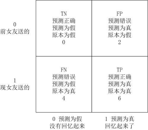
召回率 = TP / (TP + FN) = 右下 / (右下 + 左下) = 6 / (6+4) = 60%(站在现女友的角度来看)
精确率 = TP / (TP + FP) = 右下 / (右下 + 右上) = 6 / (6+2) = 75%(站在本人的角度来看)
2. 精确率。在召回率大于85%的情况下,考虑精确率
3.9 导入机器学习的库
# 逻辑回归
from sklearn.linear_model import LogisticRegression
# K折交叉验证
from sklearn.model_selection import KFold, cross_val_score
# confusion_matrix 混淆矩阵
# recall_score 计算召回率
# classification_report 显示分类指标
from sklearn.metrics import confusion_matrix, recall_score, classification_report
3.10 K折交叉验证
X_train_undersampled 拿到的是 训练集 + 验证集
对这5个recall值求平均值,得到最终的recall作为 Undersampled模型的recall值
# 测试K折验证的代码
X_try = np.array([[1,2],
                  [3,4],
                  [5,6],
                  [7,8],
                  [9,10],
                  [11,12]]) # 6行2列
# 创建KFold对象
# def __init__(self, n_splits=5, *, shuffle=False,
#                  random_state=None):
# 参数1 n_splits K折数(比如3、5等)
# 参数2 shuffle 洗牌 在拆分前是否需要把数据打乱
# 参数3 random_state 划分的结果是否随机
# 0 每次划分的结果都不同
# 1 每次划分的结果都相同
fold = KFold(n_splits=3, shuffle=False, random_state=0)
print(fold) # KFold(n_splits=3, random_state=0, shuffle=False)
# fold.split() 进行K折拆分 返回两个结果
# 返回值1 训练集
# 返回值2 验证集
for train_index, valid_index in fold.split(X_try):
    print('训练集:', train_index, ', 验证集:', valid_index)
    # 训练集: [2 3 4 5] , 验证集: [0 1]
    # 训练集: [0 1 4 5] , 验证集: [2 3]
    # 训练集: [0 1 2 3] , 验证集: [4 5]
3.11 回归算法
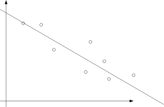
这个一般称为线性回归。目标是每个点在线上的投影,投影的模最小
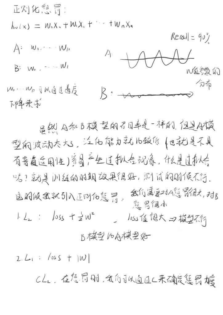
但是,很可能会导致过拟合的问题
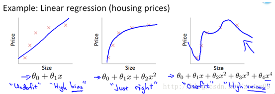
Underfit:欠拟合(High bias)
过拟合会存在的问题:在训练集上表现很好,在测试集或验证集上表现很差

简单可以w0=0,w1=0,w3=0
模型就可以简化为
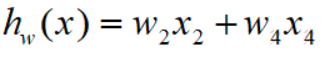
运算推算 w2=0.1 w4=0.9
这种情况一般称为正常拟合
复杂情况下,可以认为每个权值都有一点点影响
推算出 w0=0 w1=0.05 w2=0.1 w3=0.01 w4=0.84
逻辑回归
如果阶数越高,理论上对训练样本分类越准确,但是测试样本会产生过拟合的问题
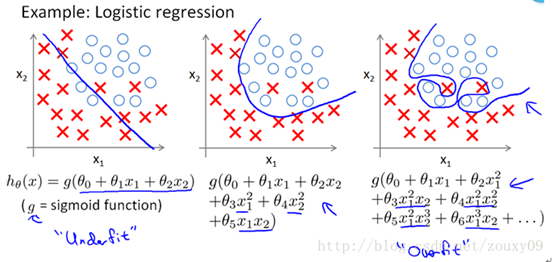
Underfit:欠拟合(High bias)
Overfit:过拟合(High varience)
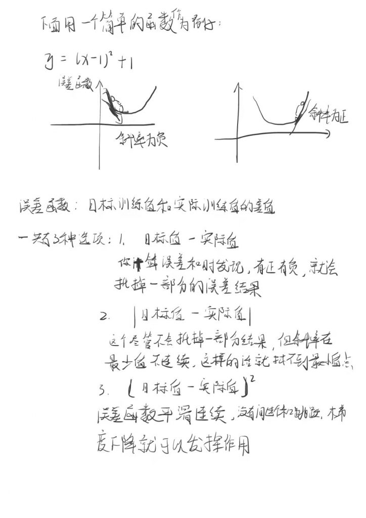
3.12 梯度下降
下山、下坡的理论
思考:这个人在什么时候可以走到最低点
一般方法求切线
当切线的倾斜度为0的时候,就认为是最低点(最值)
按照前面关于回归算法的理论,如果到达最低点,就应该属于过拟合
3.13 K折验证的函数
结合前面的几个概念:recall召回率、K折交叉验证、逻辑回归
目的是需要填写如下表:
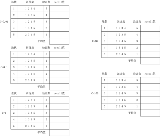
伪代码
| 遍历每个C值 对每个K值进行迭代 1 建立逻辑回归模型 2 开始训练 3 训练后需要对验证集进行预测 4 计算这次迭代的recall值 计算当前C值的平均recall值 根据各个C值的平均recall值,得到最优的C值 对应的recall即为undersampled的recall值 |
# 参数1 特征训练集+验证集 非Class项
# 参数2 结果训练集+验证集 Class项
def printing_KFold_score(x_train_data, y_train_data):
    # 对于每个C参数 都需要进行5次的交叉验证(kfold=5)
    # 创建KFold对象
    # def __init__(self, n_splits=5, *, shuffle=False,
    #                  random_state=None):
    # 参数1 n_splits K折数(比如3、5等)
    # 参数2 shuffle 洗牌 在拆分前是否需要把数据打乱
    # 参数3 random_state 划分的结果是否随机
    # 0 每次划分的结果都不同
    # 1 每次划分的结果都相同
    fold = KFold(n_splits=5, shuffle=False, random_state=None)
    # 列出一组C参数作为系数的修正(惩罚项)
    c_param_range = [0.01, 0.1, 1, 10, 100]
    # 使用pandas中的DataFrame创建5行2列的数据集
    # 参数1 data 原始的输入数据 这里不需要输入数据 因此data为None
    # 参数2 index DataFrame数据有多少行(范围) 5
    # 参数3 columns DataFrame数据有多少列(索引) 2
    # 参数4 dtype DataFrame中每条数据的数据类型
    # 参数5 是否从data中拷贝一份
    result_table = pd.DataFrame(index = range(len(c_param_range)), columns=['C参数', 'recall值'])
    j = 0 # result_table中的第几行
    # 遍历每个C参数
    for c_param in c_param_range:
        result_table.loc[j, 'C参数'] = c_param
        # 用于统计各个C参数的recall值
        recall_accs = []
        # fold.split() 进行K折拆分 返回两个结果
        # 返回值1 训练集
        # 返回值2 验证集
        iteration = 0
        for train_index, valid_index in fold.split(x_train_data):
            # 1 建立逻辑回归模型 每次交叉验证的时候都需要建立该模型 指定不同的C参数作为惩罚项
            # 参数共15个 这里只给出自己指定的参数 其他的都使用默认值
            # 参数1 penalty 惩罚项 字符串"l1"或"l2"
            # 参数4 C C参数
            # 参数9 solver 求解算法
            lr = LogisticRegression(penalty="l1", C=c_param, solver='liblinear')
            # 2 开始训练
            # 参数1 X 特征训练集
            # 参数2 y 结果训练集
            # ravel() 降维 降到一维
            lr.fit(x_train_data.iloc[train_index, :], y_train_data.iloc[train_index, :].values.ravel())
            # 3 训练后需要对验证集进行预测
            # 参数1 X 输入数据
            y_pred = lr.predict(x_train_data.iloc[valid_index, :].values)

            #print('预测结果:', y_pred)
            #print('原本结果:', y_train_data.iloc[valid_index, :].values)
            # 4 计算recall值
            #  recall_score(y_true, y_pred)
            # 参数1 y_true 真实值
            # 参数2 y_pred 预测值
            recall_acc = recall_score(y_train_data.iloc[valid_index, :], y_pred)
            iteration += 1
            print('id:', iteration, ', recall值为:', recall_acc)
            # 把当前的recall值添加到C参数对应的recall数组中
            recall_accs.append(recall_acc)
        # 计算当前C值的平均recall值
        result_table.loc[j, 'recall值'] = np.mean(recall_accs)
        print('平均的recall值为:', np.mean(recall_accs))
        j += 1

    #print(result_table)
    # 找出一个个最优的C参数
    maxval = 0
    maxid = -1
    for id, val in enumerate(result_table['recall值']):
        print('id:', id, ', C值:', result_table.loc[id]['C参数'], ', val:', val)
        if val > maxval:
            maxval = val
            maxid = id

    best_c = result_table.loc[maxid]['C参数']
    print('最优的C值是:', best_c)
    return best_c
    # 函数结束

best_c = printing_KFold_score(X_train_undersampled, y_train_undersampled)
print('最优的C值是:', best_c)
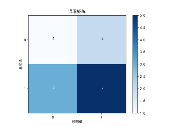
3.14 绘制混淆矩阵
使用实际的数据调用该函数
# 绘制混淆矩阵
def plot_confusion_matrix(cm, cmap=plt.cm.Blues, title='混淆矩阵'):
    # 显示二维图片
    # 共15个参数
    # 参数1 X 混淆矩阵中显示的数值 二维数组
    # 参数2 cmap 颜色 常用RGB三种颜色
    # 参数5 interpolation 插值器 常用的值
    #   nearest 最近邻插值器
    #   bilinear 双向插值器
    plt.imshow(cm, cmap, interpolation='nearest')
    # 图的标题
    plt.title(title)
    # x轴和y轴的标题
    plt.xlabel('预测值')
    plt.ylabel('真实值')
    # x轴和y轴的刻度
    plt.xticks(range(2))
    plt.yticks(range(2))
    # 显示颜色的进度值
    plt.colorbar()
    plt.rcParams['font.sans-serif'] = ['SimHei']  # 显示中文标签
    plt.rcParams['axes.unicode_minus'] = False  # 这两行需要手动设置
    # 求出cm中所有数值的最大值
    max = 0
    for i in range(2):
        for j in range(2):
            if cm[i][j] > max:
                max = cm[i][j]
    # 显示数字
    for i in range(2):
        for j in range(2):
            if cm[i][j] > max / 2:
                color = 'white'
            else:
                color = 'black'
            # 绘制文本
            # text(x, y, s, fontdict=None)
            # 参数1 x 横轴
            # 参数2 y 纵轴
            # 参数3 s 显示的文字
            # 参数color 文字的颜色
            plt.text(j, i, cm[i][j], color=color)


plt.clf() # 清空画布
cnf_matrix = [[1,2],
              [3,5]]
plot_confusion_matrix(cnf_matrix)
plt.savefig('img/2.png')
plt.show()
3.15 绘制混淆矩阵——undersampled训练集和原始数据测试集
# 1 建立逻辑回归模型
# 参数共15个 这里只给出自己指定的参数 其他的都使用默认值
# 参数1 penalty 惩罚项 字符串"l1"或"l2"
# 参数4 C C参数
# 参数9 solver 求解算法
lr = LogisticRegression(penalty="l1", C=best_c, solver='liblinear')
# 2 开始训练
# 参数1 X 特征训练集
# 参数2 y 结果训练集
# ravel() 降维 降到一维
# 注意之前是使用训练集来训练,使用验证集来预测
# 这里就应该拿训练集+验证集来训练 使用测试集来预测
lr.fit(X_train_undersampled, y_train_undersampled.values.ravel())
# 3 训练后需要对测试集进行预测
# 参数1 X 输入数据
y_pred = lr.predict(X_test.values)
# 4 计算混淆矩阵
# def confusion_matrix(y_true, y_pred, *, labels=None, sample_weight=None,
# normalize=None):
# 参数1 y_true 真实值 这里是测试集数据
# 参数2 y_pred 预测值
cnf_matrix = confusion_matrix(y_test, y_pred)
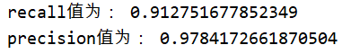
# 5 计算最终的recall值和precision值
# recall召回率: 右下 / (右下+左下)
recall = cnf_matrix[1][1] / (cnf_matrix[1][1] + cnf_matrix[1][0])
print('recall值为:', recall)
# precision精确率:右下 / (右下+右上)
precision = cnf_matrix[1][1] / (cnf_matrix[1][1] + cnf_matrix[0][1])
print('precision值为:', precision)
# 6 绘制混淆矩阵
plt.clf() # 清空画布
plot_confusion_matrix(cnf_matrix)
plt.savefig('img/4.png')
#plt.show()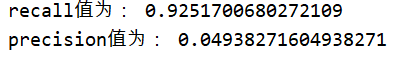
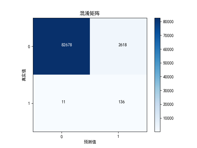
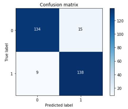
可以看到,虽然recall值还不错,但是代价是误伤太多了。很多原本是正常的交易的行为,被误认为欺诈行为。precision值太低了。
3.16 绘制混淆矩阵——原始数据训练集和原始数据测试集
不进行undersampled的操作,拿原来的样本去直接训练,看看训练的效果
# 拿原始数据进行K这交叉验证
# 需要重新计算C参数
best_c = printing_KFold_score(X_train, y_train)
print('最优的C值是:', best_c)
# 根据上面获取到的C值 重新进行逻辑回归的运算
# 1 建立逻辑回归模型
# 参数共15个 这里只给出自己指定的参数 其他的都使用默认值
# 参数1 penalty 惩罚项 字符串"l1"或"l2"
# 参数4 C C参数
# 参数9 solver 求解算法
lr = LogisticRegression(penalty="l1", C=best_c, solver='liblinear')
# 2 开始训练
# 参数1 X 特征训练集
# 参数2 y 结果训练集
# ravel() 降维 降到一维
# 注意之前是使用训练集来训练,使用验证集来预测
# 这里就应该拿训练集+验证集来训练 使用测试集来预测
lr.fit(X_train, y_train.values.ravel())
# 3 训练后需要对测试集进行预测
# 参数1 X 输入数据
y_pred = lr.predict(X_test.values)
# 4 计算混淆矩阵
# def confusion_matrix(y_true, y_pred, *, labels=None, sample_weight=None,
# normalize=None):
# 参数1 y_true 真实值 这里是测试集数据
# 参数2 y_pred 预测值
cnf_matrix = confusion_matrix(y_test, y_pred)
# 5 计算最终的recall值和precision值
# recall召回率: 右下 / (右下+左下)
recall = cnf_matrix[1][1] / (cnf_matrix[1][1] + cnf_matrix[1][0])
print('recall值为:', recall)
# precision精确率:右下 / (右下+右上)
precision = cnf_matrix[1][1] / (cnf_matrix[1][1] + cnf_matrix[0][1])
print('precision值为:', precision)
# 6 绘制混淆矩阵
plt.clf() # 清空画布
plot_confusion_matrix(cnf_matrix)
plt.savefig('img/5.png')
#plt.show()
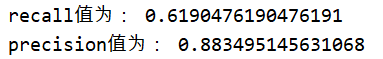
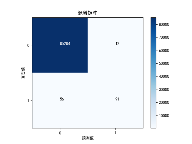
如果不做undersampled,效果就会很差。
3.17 概率和阈值
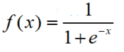
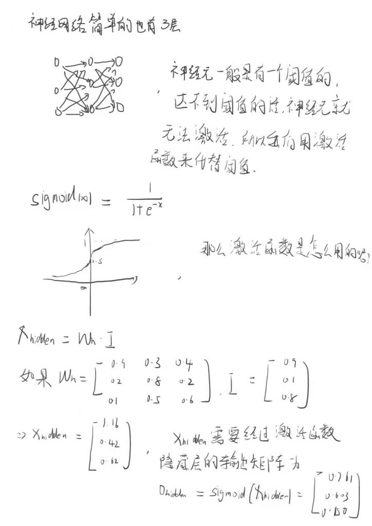
Sigmoid函数
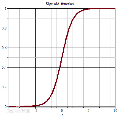
当x=0,y=0.5
当x=oo(无穷大),y=1
当x=-oo(负无穷大),y=0
留意y的范围是(0, 1),x的范围是(-oo, +oo)
Sigmoid函数的作用是把(-oo, +oo) 转换到 (0, 1),实际上就是个概率值
其实在 predict() 中,就用到 sigmoid函数
但是predict()的结果非0即1,因为给出了一个阈值。默认是0.5, 超过0.5则认为是1,小于0.5则认为是0如果根据不同的阈值绘制混淆矩阵,如下:
# 1 建立逻辑回归模型
# 参数共15个 这里只给出自己指定的参数 其他的都使用默认值
# 参数1 penalty 惩罚项 字符串"l1"或"l2"
# 参数4 C C参数
# 参数9 solver 求解算法
lr = LogisticRegression(penalty="l1", C=best_c, solver='liblinear')
# 2 开始训练
# 参数1 X 特征训练集
# 参数2 y 结果训练集
# ravel() 降维 降到一维
# 注意之前是使用训练集来训练,使用验证集来预测
# 这里就应该拿训练集+验证集来训练 使用测试集来预测
lr.fit(X_train_undersampled, y_train_undersampled.values.ravel())
# 3 训练后需要对测试集进行预测
# 参数1 X 输入数据
y_pred_undersampled_proba = lr.predict_proba(X_test_undersampled.values)
#print(y_pred_undersampled_proba) # 结果是一系列的0.0~1.0之间的值
plt.clf() # 清空画布
# 定义一系列的阈值
thresholds = [0.1, 0.2, 0.3, 0.4, 0.5, 0.6, 0.7, 0.8, 0.9]
# 遍历每个阈值
j = 1
for i in thresholds:
# 比阈值大的值 转换成1 比阈值小的值 转换成0
y_test_prediction_high_recall = y_pred_undersampled_proba[:, 1] > i
# 把9张图缩小到一张大图中
# 参数1 nrows 总共有多少行
# 参数2 ncols 总共有多少列
# 参数3 index 当前的图在第几张 1~9
plt.subplot(3, 3, j)
j += 1
# 4 计算出混淆矩阵
# 参数1 y_true 真实值 这里是测试集数据
# 参数2 y_pred 预测值
cnf_matrix = confusion_matrix(y_test_undersampled, y_test_prediction_high_recall)
# 5 计算最终的recall值和precision值
# recall召回率: 右下 / (右下+左下)
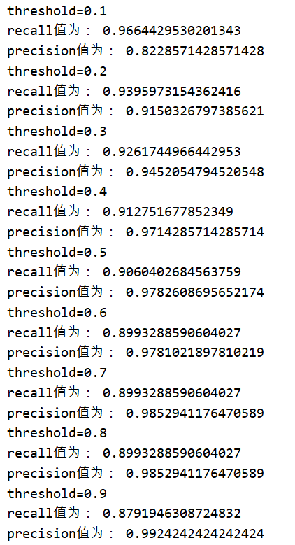
print('threshold=%.1f' % i)
recall = cnf_matrix[1][1] / (cnf_matrix[1][1] + cnf_matrix[1][0])
print('recall值为:', recall)
# precision精确率:右下 / (右下+右上)
precision = cnf_matrix[1][1] / (cnf_matrix[1][1] + cnf_matrix[0][1])
print('precision值为:', precision)
# 6 绘制混淆矩阵
plot_confusion_matrix(cnf_matrix, title='threshold=%.1f' % i)
plt.savefig('img/6.png')
plt.show()
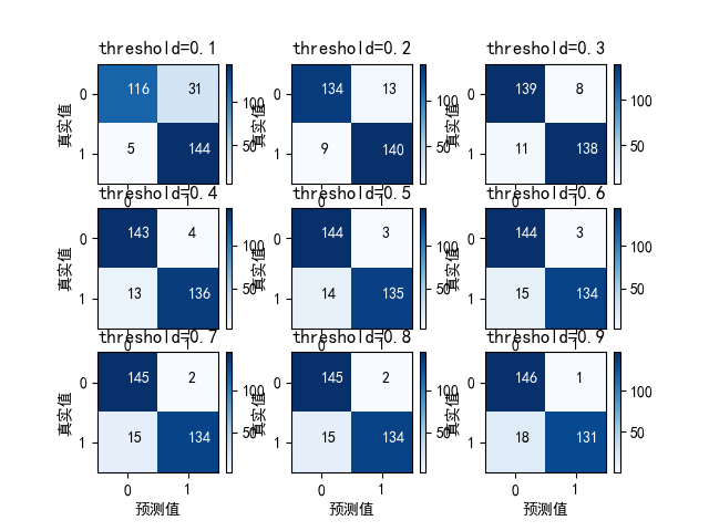
设置不同阈值时,对应的召回率recall和精确率precision
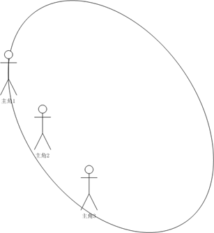
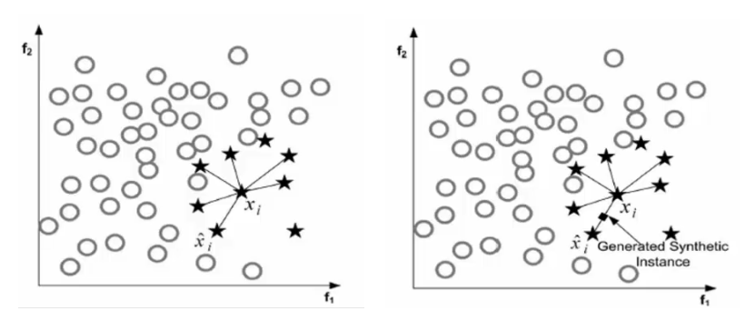
3.18 SMOTE算法
欺诈行为是492,正常行为是 284315
SMOTE算法就是无中生有,就是把欺诈行为的数量增加到和正常行为一样,原则:
1 遍历所有的少数类别样本
2 对于每个少数类型样本,找出与它最近的另一个少数类型样本(K近邻)(欧氏距离),进行连线。
3 在连线上,随机选择一点,作为新生成的点

3.19 OverSampled
首先需要安装imblearn包
pip install imblearn
pip install imblearn -i http://pypi.douban.com/simple --trusted-host pypi.douban.com
导入OverSampled所用到的包
# 导入OverSampled所用到的包
from imblearn.over_sampling import SMOTE
from sklearn.model_selection import train_test_split
# 重新对原始数据进行划分 以便后面进行测试
X_train, X_test, y_train, y_test = \
train_test_split(X, y, test_size=0.3, random_state=0)
print('对原始数据进行划分,训练集+验证集数据长度是:', len(y_train)) # 199364
print('对原始数据进行划分,测试集数据长度是:', len(y_test)) # 85443
print('总共的数据量是:', len(y_train) + len(y_test)) # 284807
3.20 生成OverSampled的样本
# 创建SMOTE对象
oversampled = SMOTE()
# 生成样本
# 参数1 X 特征训练集+验证集 非Class项
# 参数2 y 结果训练集+验证集 Class项
# 返回值1 生成的Oversampled特征训练集+验证集 非Class项
# 返回值2 生成的Oversampled结果训练集+验证集 Class项
X_train_oversampled, y_train_oversampled = oversampled.fit_sample(X_train, y_train)
print(np.sum(y_train_oversampled == 1)) # 199019
print(np.sum(y_train_oversampled == 0)) # 199019
print(y_train_oversampled.size) # 总长度 398038
3.21 计算C参数
# 对于oversampled来说 需要重新去计算C参数
best_c = printing_KFold_score(X_train_oversampled, y_train_oversampled)
print('最优的C值是:', best_c)
3.22 绘制混淆矩阵——OverSampled训练集和原始数据测试集
# 1 建立逻辑回归模型
# 参数共15个 这里只给出自己指定的参数 其他的都使用默认值
# 参数1 penalty 惩罚项 字符串"l1"或"l2"
# 参数4 C C参数
# 参数9 solver 求解算法
lr = LogisticRegression(penalty="l1", C=best_c, solver='liblinear')
# 2 开始训练
# 参数1 X 特征训练集
# 参数2 y 结果训练集
# ravel() 降维 降到一维
# 注意之前是使用训练集来训练,使用验证集来预测
# 这里就应该拿训练集+验证集来训练 使用测试集来预测
lr.fit(X_train_oversampled, y_train_oversampled.values.ravel())
# 3 训练后需要对测试集进行预测
# 参数1 X 输入数据
y_pred = lr.predict(X_test.values)
# 4 计算混淆矩阵
# def confusion_matrix(y_true, y_pred, *, labels=None, sample_weight=None,
#                      normalize=None):
# 参数1 y_true 真实值 这里是测试集数据
# 参数2 y_pred 预测值
cnf_matrix = confusion_matrix(y_test, y_pred)
# 5 计算最终的recall值和precision值
# recall召回率: 右下 / (右下+左下)
recall = cnf_matrix[1][1] / (cnf_matrix[1][1] + cnf_matrix[1][0])
print('recall值为:', recall)
# precision精确率:右下 / (右下+右上)
precision = cnf_matrix[1][1] / (cnf_matrix[1][1] + cnf_matrix[0][1])
print('precision值为:', precision)
# 6 绘制混淆矩阵
plt.clf() # 清空画布
plot_confusion_matrix(cnf_matrix)
plt.savefig('img/7.png')
#plt.show()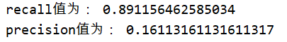

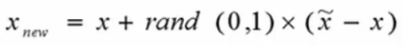
精确率大概是 16.1%(比较underampled精确率只有4.9%)结论是:使用 oversampled 训练的效果比 undersampled 要好当然,oversampled 花费的时间也比较多
数据量多,花的时间多,训练出来的模型更准确
3.23 结论
对于误伤的情况,银行一般会使用人工的方式进行复查。打电话逐个询问(这个是不是你的交易)
作业:根据实际的运行情况,自己给出该案例模型训练的结论。
3.24 讲义
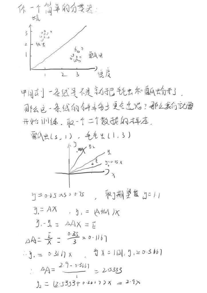
是不是发现这两条直线跳动的幅度太大了,这时候我们加入调节系数L

L*(E/X),然后再计算下
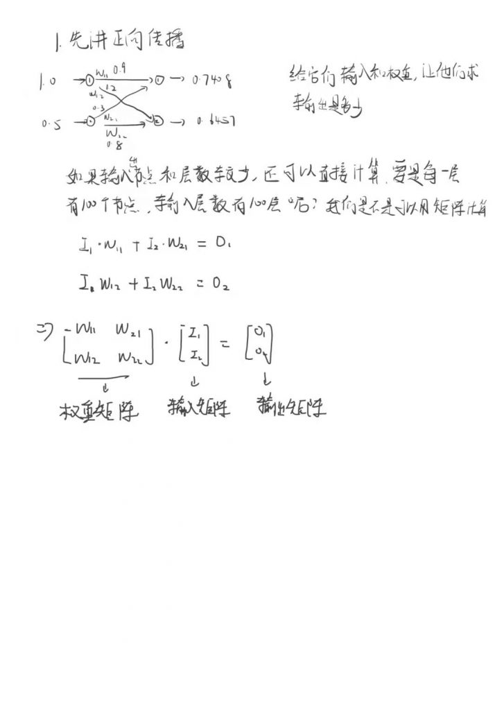
然后再用隐藏层的输出当做输出层的输入,在和这部分的权重矩阵相乘就得到了最终的输出。
得到输出之后和和我们的目标值肯定不一样,然后我们就他们做一个差值,计算出误差的大小。
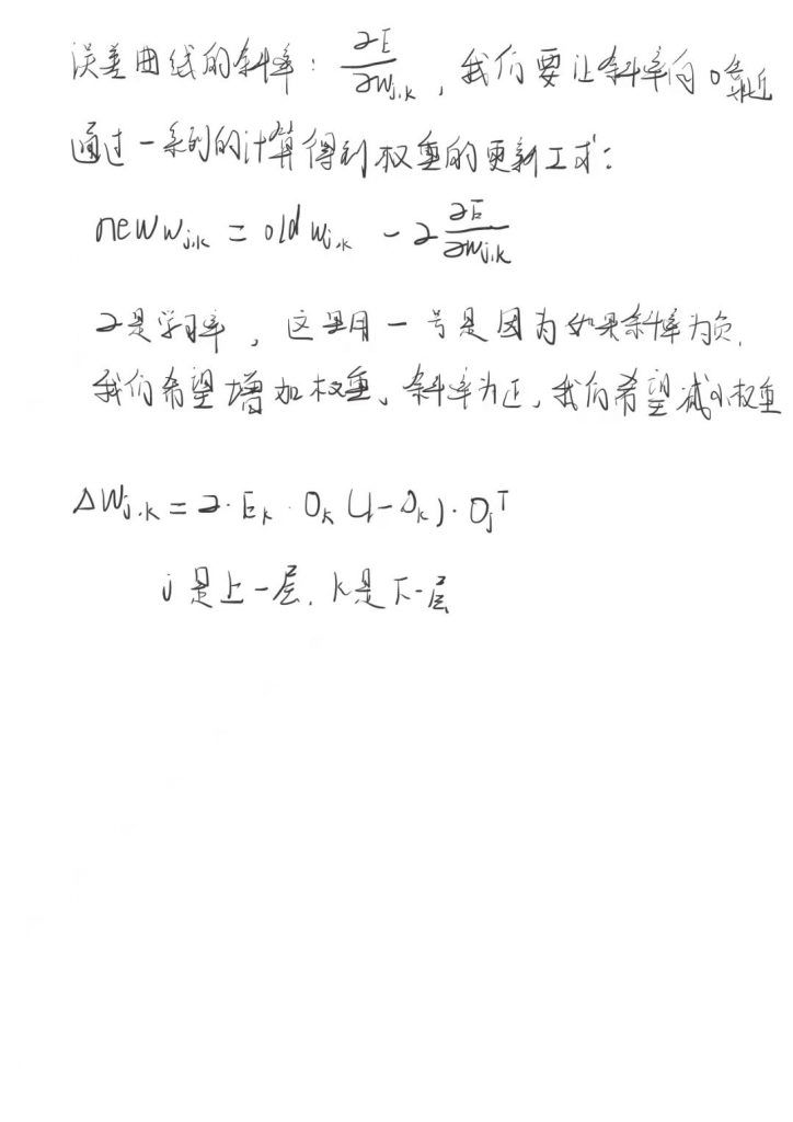
知道误差大小后我们怎么重新更新权重参数让误差更小,这时候得讲到反向传播
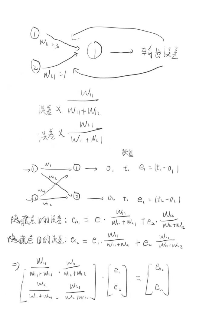
知道误差了,那我们如何更新权重让误差更小呢,这时候就要讲到一个梯度下降的方法